Edward Conard

Top Ten New York Times Bestselling Author

  • “…a must-read for serious students of economic policy.” - Glenn Hubbard, Dean, Columbia Business School, and former Chairman of the Council of Economic Advisers
  • “…a fresh argument for the productive value of inequality.” - David Autor, Professor of Economics, Massachusetts Institute of Technology
  • “…a comprehensive explanation of the modern economy.” - Julian Robertson, Founder, Tiger Management
  • “Unintended Consequences offers deep and well-argued analyses on almost every issue.” - The New York Times
  • “…challenges misconceptions that distort our economic debates.” - Arthur Brooks, President of the American Enterprise Institute
  • “Unintended Consequences is far smarter and more thought-provoking than most economics written for the general public” - Greg Mankiw, Harvard University, Former Chairman of the Council of Economic Advisors
  • “…serious thinking for serious thinkers. …a thought-provoking blueprint for growing middle- and working-class incomes.” - Mitt Romney, former Governor of Massachusetts
  • “…challenges misconceptions that distort our economic debates.” - Arthur Brooks, President of the American Enterprise Institute
  • “…a fresh argument for the productive value of inequality.” - David Autor, Professor of Economics, Massachusetts Institute of Technology
  • “A full-throated defense of economic dynamism.” - The Wall Street Journal
  • “…serious thinking for serious thinkers. …a thought-provoking blueprint for growing middle- and working-class incomes.” - Mitt Romney, former Governor of Massachusetts
  • “…a very valuable contribution.” - Larry Summers, former Secretary of the Treasury and director of the National Economic Council, president emeritus, Harvard University
Upside of Inequality Oxford Unintended Consequences
Buy the Books
  • Macro Roundup
  • About Roundup
  • About Ed Conard
  • Highlights
  • Topics
  • Subscribe
Edward Conard
  • twitter
  • facebook
  • linkedin
  • youtube

Macro Roundup

  • Email
  • Text Message (SMS)
  • Twitter/X
  • LinkedIn
  • Facebook
  • WhatsApp Message
Subscribe to Macro Roundup Emails
Select topics to choose: articles that mention them (broader) or articles mainly about them (focused)
  • Mentions 0
  • Primary focus 0
Showing all 7,294 Macro Roundup articles
When you search for any topic (like GDP, Inflation, or Banking), choose:
Choose search scope

Monday, July 18, 2022

How a Public School in Florida Built Americas Greatest Math Team

AI Summary. Buchholz High School in Florida has won 13 of the last 14 national math championships using a curriculum that emphasizes speed, pattern recognition, and efficient problem-solving, identifies talent early, and integrates four levels of instruction. Its average margin of victory rose from 315 to 920 points, while the U.S. ranks 37th in international math rankings.

Ben Cohen Wall Street Journal
Date Posted:
July 18, 2022
Is Database:
Database

Buchholz High School in Florida has achieved remarkable success by prioritizing speed over accuracy in math education, winning 13 of the last 14 national math championships.

How can a public school build a dominant national math team?

Core argument: Buchholz High School in Florida has won 13 of the last 14 national math championships, with its average margin of victory rising from 315 to 920 points.

Buchholz High School in Florida has achieved remarkable success by prioritizing speed over accuracy in math education, winning 13 of the last 14 national math championships. This approach contrasts with the U.S.'s overall decline to 37th in international math rankings. Mr. Frazer, a former Wall Street bond trader, implemented a curriculum emphasizing pattern recognition and efficient problem-solving, allowing students to solve complex problems quickly. By identifying talent early and integrating four levels of education, Buchholz has created a pipeline of math talent. The program's success is evident in its national titles, with the average margin of victory increasing from 315 to 920 points. This model, which combines competitive spirit with innovative teaching methods, could serve as a blueprint for improving math education nationwide.

Takeaways by Macro Roundup® AI

  1. Buchholz High School in Florida has won 13 of the last 14 national math championships, with its average margin of victory rising from 315 to 920 points.
  2. Mr. Frazer, a former Wall Street bond trader, built Buchholz's curriculum around speed over accuracy, pattern recognition, and efficient problem-solving, identifying talent early and integrating four levels of education into a math talent pipeline.
  3. Buchholz's record stands against an overall U.S. decline to 37th in international math rankings, and its model could serve as a blueprint for improving math education nationwide.

Note the University of Florida is in Gainesville - so the teacher is likely just teaching the professors kids, “…I wanted to understand how this otherwise average public high school in Florida had managed to win 13 of the last 14 national math championships. The extraordinary thing about the Buchholz math team is how ordinary Buchholz is. It’s ranked 66th among schools in Florida and outside the top 1,000 across the country, according to U.S. News & World Report. But at the annual championships of Mu Alpha Theta, the national math honor society, the Buchholz kids have trouble counting the shiny objects they lug home…The big difference between a traditional honors class and Mr. Frazer’s class is the way students learn to approach tricky problems. He teaches accuracy, but he also teaches speed, since competitive tests are timed. He believes that pattern recognition is a more useful skill—in math, and in life—than cloning questions his students might have seen on their homework the night before. Here’s a basic example involving a famous math problem: What’s the sum of every integer from 1 to 100? You could answer the question with brute force and punch all those numbers into a calculator, but students who are trained to think outside the box would instinctively look for symmetry. They would see that pairs of 1+100 and 2+99 and 3+98 add up to the same total and would simply multiply 101 by 50. They get the correct answer of 5,050 in a fraction of the time. “Everyone has this idea that we practice constantly,” Mr. Frazer said as his students plowed through problem sets on their summer vacation. “It’s not true. We use our time efficiently.”…”

Ben Cohen, "How a Public School in Florida Built America’s Greatest Math Team,"Wall Street Journal, July 14, 2022, https://www.wsj.com/articles/the-secrets-of-americas-greatest-high-school-math-team-11657791000

How a Public School in Florida Built America’s Greatest Math Team

GAINESVILLE, Fla.—It was a sticky Thursday afternoon in the middle of summer break when dozens of teenagers walked through the doors of their high school. One of the world’s most dominant teams was about to start math practice.

There was probability in one classroom and pre-algebra next door, code-breaking down the hall and number theory around the corner. And there were few adults to be found anywhere. The students would spend the rest of the day teaching each other.

I had also come here to learn from them. I wanted to understand how this otherwise average public high school in Florida had managed to win 13 of the last 14 national math championships.

The Buchholz High School math team is a dynasty built by one teacher with a strategy for identifying talent, maximizing potential and optimizing the American system of education.

Will Frazer popped out of his flaming red Corvette as his students were trickling into the classrooms. A bond trader on Wall Street in the 1980s, Mr. Frazer retired young and moved to Florida, where he became a scratch golfer and lived the dream for a decade. Then he got bored.

He took a job at Buchholz coaching golf, switched to teaching math, quickly formed a math team, applied the lessons of his experience in finance and turned a bunch of teenage quants into a fearsome winning machine.

“The difference between what I do now and what I did on Wall Street is that I used to get paid money,” said Mr. Frazer, 63. “Now we get trophies.”

The extraordinary thing about the Buchholz math team is how ordinary Buchholz is. It’s ranked 66th among schools in Florida and outside the top 1,000 across the country, according to U.S. News & World Report. But at the annual championships of Mu Alpha Theta, the national math honor society, the Buchholz kids have trouble counting the shiny objects they lug home.

Buchholz is an outlier in more ways than one. The math team’s run since 2007 coincides with the U.S. slipping to 37th place in the latest international rankings of teenage math performance and China starting to produce more STEM doctorates than American universities for the first time.

The son of an economist, Mr. Frazer believes in competition. He refuses to call the Buchholz math students a club because he wants them to think of themselves as a team. “A club is a social organization,” he said. “A team comes together to win.” And he was out to win.

As he picked the brains of rival coaches whose teams consistently beat Buchholz, Mr. Frazer became obsessed with one question: Why were their kids better at math?

It was because they were teaching math in an entirely different way.

“Here’s the typical model at every school,” he said. “You teach the kids the boring honors stuff during the day, and then you come after school to practice the competitive stuff.” What he meant by the boring honors stuff was the rote memorization and regurgitation that makes Mr. Frazer want to eat his calculator. “Life is not like that,” he said.

The trader in Mr. Frazer saw an inefficiency that he could exploit.

“My thought was I should find out what the best are doing and then figure out what the flaw in the model is,” he said.

With the backing of his school principal and the cooperation of his superintendents, he set about overhauling the Buchholz math department, implementing his own curriculum and hunting for talent at younger ages.

He believes the pipeline for the high school’s math team must begin long before students reach high school, so Mr. Frazer searches for prospects in elementary school and steers them to accelerated math classes in middle school.

“You wouldn’t grab a kid in ninth grade who’s never played football and expect him to be a great high-school football player,” he said. “For most of these kids, this is their football.”

Mr. Frazer’s insight was to connect four levels of education: The kids he scouts in elementary school develop in middle school, compete in high school and take specialized classes from college professors that he brings to Buchholz’s campus. As soon as the system was in place, the team started winning and never stopped.

It turned out there was value in putting a bunch of smart kids in the same room: They feel empowered to make each other smarter.

Many of the gifted kids in his program have parents who work at the nearby University of Florida and push to get on Mr. Frazer’s radar. Others he finds on his own. He tracks down test scores of students in his district, follows the data and recruits high achievers. Some who were discovered by his spreadsheets have since graduated from the Massachusetts Institute of Technology with math degrees and landed on Wall Street themselves.

The mathletes who try out for the team and make the cut are combined into one class section and fly through competitive algebra, geometry and calculus during the school day. Mr. Frazer essentially bends the rules to move faster through harder material and pack more than two years of math into one school year. “I cover everything the state wants me to cover,” he said. “But there is no restriction on covering extra material.”

How a Public School in Florida Built Americas Greatest Math Team: Extended Excerpt Image 1


The big difference between a traditional honors class and Mr. Frazer’s class is the way students learn to approach tricky problems. He teaches accuracy, but he also teaches speed, since competitive tests are timed. He believes that pattern recognition is a more useful skill—in math, and in life—than cloning questions his students might have seen on their homework the night before.

Here’s a basic example involving a famous math problem: What’s the sum of every integer from 1 to 100? You could answer the question with brute force and punch all those numbers into a calculator, but students who are trained to think outside the box would instinctively look for symmetry. They would see that pairs of 1+100 and 2+99 and 3+98 add up to the same total and would simply multiply 101 by 50. They get the correct answer of 5,050 in a fraction of the time.

“Everyone has this idea that we practice constantly,” Mr. Frazer said as his students plowed through problem sets on their summer vacation. “It’s not true. We use our time efficiently.”

That means taking advantage of an opportunity hiding in plain sight: the summer. Hundreds of students come to school four hours a day, five days a week for a month during vacation. It adds up to 80 hours of extra practice.

There was a buzz inside Mr. Frazer’s classroom when I was there because the teacher at the whiteboard was charismatic—and she wasn’t Mr. Frazer.

Instead, a high-school sophomore named Katie He was instructing middle-schoolers, one of Mr. Frazer’s methods for pulling off a feat that many consider impossible: making math fun.

It’s a universal truth of childhood that nothing is cooler than being around someone a few years older. They may be there because of their parents, but they stick around because of their peers. The younger kids want to impress the students they idolize, and the high-schoolers are compensated for their time in community-service hours. The model is cheap, innovative and wildly effective. It’s as if Billy Beane were running a math team.

Timothy Jin, a rising Buchholz sophomore, wasn’t exactly thrilled by the idea of waking up early for summer math while in middle school. “I obviously thought, like, ‘Oh, it’s going to be another boring math class,’” he said. But he soon realized how wrong he was. Now he’s a teacher at the camp.

Hailey Lin knows how it sounds when people hear about math practice. “But it’s not, like, ‘Oh, my God, I have to do math,’” the Buchholz junior said. She loves the collaborative elements of team competitions and challenging herself against the best of the best. “I thought I was really good at math,” she said. “Then I came here.” (Mr. Frazer described her as one of the best female math students in the country.)

For someone always on the lookout for the latest edge, the pandemic unexpectedly presented Mr. Frazer with one. After the school shutdowns in early 2020, he feared more disruptions in 2021, so he made a curious decision: He resigned from Buchholz—and he kept teaching.

How a Public School in Florida Built Americas Greatest Math Team: Extended Excerpt Image 2


He rented an empty wing of his church and told parents that he would be teaching his usual curriculum in person as if it were a normal school year. Their kids could learn from him and take the rest of their classes remotely or carpool back and forth to Buchholz. Mr. Frazer says he invited 145 students. His friends thought 20 or 30 would come with him. His pastor was optimistic and predicted 80. He got 140.

The math team proceeded to win last year’s state and national titles by the widest gaps in the history of the program. The average margin of victory in Buchholz’s previous national titles was 315 points. Last year, it won by 920.

Total freedom from bureaucracy was tempting, but Mr. Frazer missed school enough to return to Buchholz and his old classroom right in time for politicians around the state to pay attention.

“The Buchholz math program should serve as a national model for other schools and districts to follow,” Florida education commissioner Manny Diaz Jr. said.

Buchholz is trying to beat them first. There was math to be done and trophies to be won at the Mu Alpha Theta convention this week in Washington, D.C., where Mr. Frazer bused 70 students for team events and individual subjects ranging from probability and combinatorics (“Prob & Combo”) to differential equations (“Diffy Q”). The star of the team this year happened to be his elder son, Jake, who’s off to college next month, but there were younger whizzes like Ms. He, Mr. Jin and Ms. Lin among the hundreds of students in quiet rooms attacking exams with their pencils.

Mr. Frazer spent years trying to crack the code for making students better at math. He’s still working on it. But one measure of his success is that the best kids on his team are now better than he is.

“Every kid at Alabama is better than Nick Saban at football,” Mr. Frazer said of the legendary coach with the most college national championships. “He just knows how to win better than anyone on the planet.”

By the time their buses were on the road back to Florida, the Buchholz math team had been crowned national champions. Again.

  • Test Scores
  • Workforce
    • Education
      • K-12

Why Canada Should Pay More for Medications

AI Summary. Removing pharmaceutical price controls across developed economies is estimated to raise development of new drugs by 9-12% by 2030 and extend life expectancy for today's 15-year-olds by up to 1.6 years. The U.S. funds 44% of global pharmaceutical research spending and produces 40% of patented drugs, while Canada's prices are nearly 3.5x lower and it ranks 27th in pharmaceutical innovation.

Richard Owens Wall Street Journal
Date Posted:
July 18, 2022
Is Database:
Database

Removing price controls in OECD countries could boost new pharmaceuticals by 9-12% by 2030, extending life expectancy for today’s 15-year-olds by up to 1.6 years @RichardOWens @WSJ.

Removing price controls in OECD countries could boost new pharmaceuticals by 9-12% by 2030, extending life expectancy for...

Would ending drug price controls abroad boost innovation and life expectancy?

Core argument: Removing price controls across OECD countries could raise development of new pharmaceuticals by 9–12% by 2030 and extend life expectancy for today's 15-year-olds by up to 1.6 years.

The removal of price controls in OECD countries could boost the development of new pharmaceuticals by 9-12% by 2030, potentially extending life expectancy for today's 15-year-olds by up to 1.6 years. Currently, the U.S. shoulders 44% of the global R&D budget for pharmaceuticals, producing 40% of the world's patented drugs, while price-controlled countries like Canada benefit from lower prices at the expense of innovation. Canadian prices are nearly 3.5 times lower than in the U.S., yet Canada ranks only 27th in global pharmaceutical innovation. Increasing drug prices in Europe by 20% could yield $17.5tn in welfare gains for both the U.S. and Europe. A coordinated effort to reform international pharmaceutical pricing could alleviate pressure on the U.S. market and ensure equitable cost-sharing, fostering a more innovative and sustainable global pharmaceutical industry.

Takeaways by Macro Roundup® AI

  1. Removing price controls across OECD countries could raise development of new pharmaceuticals by 9–12% by 2030 and extend life expectancy for today's 15-year-olds by up to 1.6 years.
  2. The U.S. bears 44% of the global pharmaceutical R&D budget and produces 40% of the world's patented drugs, while price-controlled countries such as Canada pay less at the expense of innovation.
  3. Canadian drug prices are nearly 3.5 times lower than U.S. prices, yet Canada ranks 27th in global pharmaceutical innovation, and raising European prices by 20% could yield $17.5tn in welfare gains for the U.S. and Europe.

“…Robbed of revenue by price controls, pharmaceutical companies find it where they can—the U.S. The American consumer pays high prices to support research and development that benefits the world. The U.S. invests 44% of the world’s R&D budget for pharmaceuticals, and produces the largest share of patented pharmaceuticals, at any given time accounting for some 40% of the world’s patented drugs…. It has been estimated that if OECD countries lifted their price controls, the number of new pharmaceuticals that would be developed would increase by between 9% to 12% by 2030. This could extend life expectancy of today’s 15-year-olds by up to 1.6 years. To increase prices in price-controlled European countries by only 20% would lead to $17.5 trillion in combined welfare gains for the U.S. and Europe alike….”

Richard Owens, "Why Canada Should Pay More for Medications,"Wall Street Journal, July 17, 2022, https://www.wsj.com/articles/canada-should-pay-more-for-medications-price-controls-oecd-innovation-prescription-drugs-revenue-prices-pharmaceuticals-11658084406

Why Canada Should Pay More for Medications

American lawmakers are threatening to impose price controls on prescription drugs, and it isn’t hard to see why. We Canadians, like others outside the U.S., get our medications at bargain prices—and at the expense of the American consumer, who pays full freight and then some. Americans are tired of free riders, and they deserve a break.

But there’s no way to maintain the vehicle if everyone rides free. U.S. price controls would perhaps benefit consumers in the short term, but at the cost of killing innovation. The only solution is for Canada and other countries to step up and accept their fair share of the cost.

The Patented Medicine Prices Review Board administers Canada’s price controls, forcing drugmakers to sell at a deep discount. Prices of patented pharmaceuticals are almost 3.5 times as high in the U.S. as in Canada. Even so, Canadian prices are among the highest in the Organization for Economic Cooperation and Development—but all non-U.S. members of the 38-country OECD cluster in a narrow pricing band far below America.

Consumers outside America do pay a price for this, as new drugs reach the market more slowly if at all. At any given time, U.S. pharmacies can sell some 90% of available patented pharmaceuticals, compared with about 47% across price-controlled countries (this figure is somewhat higher, 65%, in Canada).

Price controls depress investment for research and development. Out of 56 countries ranked for their contributions to global pharmaceutical innovation, the U.S. ranks first while Canada ranks 27th. A profitable pharmaceutical industry benefits everyone, because R&D spending grows in proportion to profits. More R&D means more new pharmaceuticals, more years of life and health, and less spending on expensive nonpharmaceutical treatments. But the pharmaceutical industry isn’t especially profitable. Automobiles, financial services, information technology and other industries earn far more return on equity.

Robbed of revenue by price controls, pharmaceutical companies find it where they can—the U.S. The American consumer pays high prices to support research and development that benefits the world. The U.S. invests 44% of the world’s R&D budget for pharmaceuticals, and produces the largest share of patented pharmaceuticals, at any given time accounting for some 40% of the world’s patented drugs.

If a country exported a product at a below-market subsidized price to benefit its own producers, it could face a dumping complaint to the World Trade Organization. Trade law has no remedy for price controls by importing countries. But the U.S. could make proportional price reduction for the U.S. consumer a quid pro quo for allowing other nations to import its innovative pharmaceuticals. It could impose export fees equivalent to some or all of the lost wholesale pricing attributable to price controls.

To lower prices again, countries with price controls would have to get together to effect an equitable sharing of price increases in their more open markets. The U.S. could also bring foreign drug producers to support local price reform by implementing a rule requiring that no drug in the U.S. sells for more than it sells in its exporting jurisdiction.

The cost of low drug prices is high for everyone. It has been estimated that if OECD countries lifted their price controls, the number of new pharmaceuticals that would be developed would increase by between 9% to 12% by 2030. This could extend life expectancy of today’s 15-year-olds by up to 1.6 years. To increase prices in price-controlled European countries by only 20% would lead to $17.5 trillion in combined welfare gains for the U.S. and Europe alike.

The world desperately needs international pharmaceutical pricing reform, but there’s a collective-action problem. The cost for Canada or any other single nation to go cold turkey on price controls would be prohibitive. But if nations act in concert, pressure on the U.S. market could be relieved and price increases in local markets managed. Canada and other OECD countries aren’t poor. It’s time for us to pay our share.

  • Productivity
    • Incentives/Risk-Taking
    • Innovation/Research
    • Institutional Capabilities
    • Investment
  • Fiscal Policy
    • Regulation

Thursday, July 21, 2022

Short-Term Tax Cuts, Long-Term Stimulus NBER

AI Summary. Corporate income tax cuts are estimated to produce persistent increases in research and development spending, productivity, and real GDP, with a 0.5% GDP gain lasting over a decade and effects peaking around eight years out. Personal income tax cuts, by contrast, generate large boosts to output and productivity that dissipate within two years.

James Cloyne National Bureau of Economic Research
Date Posted:
July 21, 2022
Is Database:
Database

Corporate income tax cuts lead to significant & persistent increases in R&D spending & productivity, with effects peaking around 8 years post-shock. In contrast, personal income tax cuts yield large but short-lived boosts to output & productivity.

Do corporate tax cuts boost long-run growth more than personal tax cuts?

Core argument: Corporate income tax cuts raise real GDP by 0.5%, with the increase persisting over a decade alongside gains in R&D spending and productivity that peak roughly eight years after the shock.

Corporate income tax cuts, while initially modest in impact, lead to significant and persistent increases in R&D spending and productivity, with effects peaking around eight years post-shock. This sustained R&D response is a key driver of long-term GDP growth, as evidenced by a 0.5% increase in real GDP persisting over a decade. In contrast, personal income tax cuts yield large but short-lived boosts to output and productivity, with effects dissipating within two years. The disparity in outcomes is further highlighted by the fact that corporate tax changes have larger long-term effects on GDP and productivity in 93% and 98% of cases, respectively, compared to personal tax changes. This suggests that corporate tax policy is more effective for long-term economic stimulus through its influence on innovation and productivity.

Takeaways by Macro Roundup® AI

  1. Corporate income tax cuts raise real GDP by 0.5%, with the increase persisting over a decade alongside gains in R&D spending and productivity that peak roughly eight years after the shock.
  2. Personal income tax cuts deliver large boosts to output and productivity that dissipate within two years, unlike the persistent effects of corporate tax cuts.
  3. Corporate tax changes produce larger long-term effects than personal tax changes on GDP in 93% of cases and on productivity in 98% of cases.

Key Finding, "..Do transitory changes in corporate and personal income taxes have persistent effects on output? And what are the channels?The effects of personal income taxes on output are large and significant during the first six quarters but return to zero within two years. In contrast, a corporate income tax cut generates a smaller stimulus on impact but has larger expansionary effects over the medium- and long-term, with peak effects occurring around eight years after the shock.Variable factor utilization is crucial to produce the short-run response of productivity. While the dynamic effects of personal income taxes are short-lived on productivity and negligible on R&D expenditure, changes in corporate income taxes are associated with a sustained, but temporary, rise in R&D spending and a persistent increase in aggregate productivity. R&D is key for the model’s ability to generate a persistent response of productivity and output following a temporary change in corporate income taxes. A standard New-Keynesian model would not deliver pro-cyclical productivity, thereby missing the estimated output responses to either shock...."
The Evidence

“…Using the approach outlined above, we now present our baseline set of empirical estimates about the longer-term effects of cuts to corporate and personal income taxes. We first focus on the response of the average tax rate, GDP and productivity, with the latter being a key and novel focus of our analysis. We will then extend our empirical evidence to examine investment, R&D and consumption to shed light on the most likely mechanism driving the GDP responses. Each further variable is added to the benchmark data vector Z one at the time to avoid a sharp increase in the number of parameters to be estimated. In Figure 1, we present our first set of main results. The figure contains two columns. On the left, we show the IRFs to a reduction in the average corporate tax rate. On the right, we show the results for a reduction in the average personal tax rate. The impact effect is normalized so that both shocks reduce their respective average tax rate by 1 percentage point in the first period. The solid red lines are the posterior medians and the shaded bands refer to 68% and 90% (Bayesian) credible intervals. Impulse response functions are computed using posterior draws of the coefficients A0 and B1. The solid blue lines come from the estimated structural model that will be presented, solved and estimated in Section 5. The first row in Figure 1 reveals that, following a shock to corporate and personal income taxes, the average tax rates decline temporarily. The change in the average corporate tax rate (first column) loses significance after 8 quarters and goes back to zero after around 20 quarters. The changes in the average personal income tax rate are somewhat less persistent, losing significance after 6 quarters and touching zero after around 16 quarters. Despite the different method (i.e. local projections vs. VAR), these results largely replicate the findings in Figures 2 and 3 of Mertens and Ravn (2013), where the results are plotted for the first 20 quarters. In short, the estimated tax cuts are rather transitory….”

Short-Term Tax Cuts, Long-Term Stimulus NBER: Extended Excerpt Image 1


“…The second row in Figure 1 shows the impulse response functions for the percentage response of real GDP. As expected, the IRFs for the first 20 quarters are very comparable to the main figures in Mertens and Ravn (2013). What is new is our estimate of the longer-term effects beyond quarter 20. Looking at the first column it is clear that, despite the transitory nature of the corporate tax reduction, there are very persistent effects on real GDP, whose short-run increase of 0.5% persists throughout the ten year period shown in the figure. In other words, the corporate income tax cut has disappeared after 5 years, but the effect on the level of economic activity is still sizable and significant after 8 years. The second column, however, reveals that the average personal tax rate cut does not produce such long-lasting dynamics.The underlying personal income tax cut is only slightly more transitory than the corporate tax cut but its effects on GDP are far less persistent and appear to die out already after two to three years after the shock hits. A similar picture emerges for productivity, as shown in the third row of Figure 1. Both tax rate cuts boost productivity on impact, with the size of the initial response to a personal income tax cut being much larger than for a cut to corporate taxes. On the other hand, the effects of corporate tax cuts grow over time and remain significant even after 10 years. In sharp contrast, the response of productivity to a change in personal income tax rates is not statistically different from zero already after two years. The clear difference in the short-run and long-run properties of the two taxes can be illustrated further by looking at the joint posterior distribution of transitory and persistent responses of the variable of interest in Figure 2.The top row refers to GDP while the bottom row represents productivity. We use ‘transitory’ (or shorter-term) to mean the effect estimated within 2 years after the shock, while ‘persistent’ (or longer-term) represents the dynamic effects estimated beyond the two year horizon The horizontal axis shows the response to a corporate tax cut, while the vertical axis shows the associated responses to a personal income tax cut. For the sake of exposition, each panel also reports the 45o degree line, which is the locus of points where the effects of personal and corporate income taxes on the variable of interest are numerically identical. Posterior draws below (above) the 45o degree line indicate a larger impact of corporate (personal) taxes. The share of draws below the 45o degree line, which we denote as δ in Figure 2, can therefore be seen as a measure of the probability that corporate tax changes have larger effects. In Appendix Figure A.2, we show that our flat priors for the LP parameters imply very disperse joint prior distributions for the short-run and long-run effects of the two shocks on GDP and productivity. These joint prior distributions are centered at (0,0). As a result, there is an even chance that the (persistent and transitory) effects of one type of tax will dominate the other. The left column indicates that for only about 6% of posterior draws do corporate income tax changes have larger short-term effects on GDP (top row) and productivity (bottom row) than personal income tax changes. In sharp contrast, the right column of Figure 2 reveals that corporate income tax cuts have significantly larger long-term effects than personal income tax cuts in about 93% of posterior draws for GDP and 98% for productivity. We conclude that the evidence of heterogeneous responses across both forecast horizons and type of income tax in Figure 1 is significant at conventional levels…”

Short-Term Tax Cuts, Long-Term Stimulus NBER: Extended Excerpt Image 2


“…In Appendix A3, we report the responses of Total Factor Productivity (TFP), total hours and employment. Our theoretical model will not, however, feature an extensive margin so the employ- ment IRF will not be used in the structural estimation in Section 5. The three main takeaways from this additional analysis are that: (i) the response of total hours and employment to a corporate income tax cut is typically modest and insignificant; (ii) in contrast, changes in personal income taxes have a significant but short-lived impact on total hours but muted effects on employment; (iii) the effects on TFP are very similar to those based on labour productivity. In summary, in the short-run, the effects of personal income tax changes on output, productivity and hours worked are significantly larger than the effects of corporate income tax changes. Over longer horizons, however, the responses of output and productivity to corporate income tax cuts are large and highly significant. In contrast, the long-run effects of a personal income tax cut are indistinguishable from zero, both in economic and statistical terms. In the next section, we will extend our empirical analysis to investment, R&D expenditure and consumption in an effort to shed light on the possible mechanism behind the heterogeneity documented in Figure 1 and Figure 2….”

The Mechanisms

“….The impulse responses in Figures 1 and 2 replicate the results in Mertens and Ravn (2013) over the first 20 quarters, which is the horizon at which most previous literature stops. On the other hand, we have shown that there are significant longer-term effects of corporate tax cuts that persist beyond the typical IRF horizons presented in earlier work. These persistent dynamics are not, however, evident for the effects of personal tax cuts. In the rest of the paper we investigate what may explain these findings. In this sub-section, we look at a number of additional variables that could offer insights on the transmission mechanism, especially at longer horizons. These are R&D expenditure, investment and consumption expenditure. The endogenous growth literature argues that R&D spending has the potential to generate persistent effects on both output and productivity. On the other hand, studies in the Real Business Cycle tradition emphasize the role of capital expenditure as an important propagation mechanism. Finally, given such longer-term output responses, we would also expect to see persistent effects on household expenditure for corporate tax changes, with short-lived effects from personal tax changes. The findings are reported in Figure 3. The first row shows the impulse responses of R&D expenditure to a corporate tax cut (left column) and to a personal tax cut (right column). The second and third rows show the dynamic effects on investment and consumption respectively. Red lines represent medians and 68% credible sets of the impulse response posterior distributions. Shaded areas refer to 90% central intervals. As discussed in Section 2, each variable is added one at the time to our baseline dataset to avoid a sharp increase in our already richly parameterized local projections….”

Short-Term Tax Cuts, Long-Term Stimulus NBER: Extended Excerpt Image 3


“…The evidence in the first row of Figure 3 suggests that the effects of corporate tax cuts (first column) on R&D are initially negligible but become significant at about one year after the shock. The increase is persistent and reaches a peak of 1.4% at quarter 18 before returning to zero after nine years. The effect also loses significance after six years. The response of investment to corporate tax changes (second row) is equally strong but its significance seems more short-lived. Finally, the consumption profile (third row) is similar to the pattern of the impulse responses of output and productivity in Figure 1.The significant and sustained rise in R&D seems a plausible candidate for explaining the persistent increase in productivity reported in Figure 1. In the next sections, we will explore this conjecture formally by developing and estimating a structural model with endogenous growth via R&D. The estimated effects of a personal income tax cut (second column of Figure 3), paint a different picture. The response of R&D is never statistically different from zero while the change in investment is larger but far more transitory than for corporate tax changes. The effects on R&D and capital expenditure suggests that the sharp and short-lived increase in productivity after a personal income tax cut in Figure 1 does not come from firms’ innovation activities. Later, we show that this is consistent with a short-run labor utilization story. Finally, the response of consumption in the bottom row largely inherits the shape of the GDP profile, as was the case for corporate taxes. This is consistent with the notion that corporate taxes raise labor income persistently, while personal taxes affect incomes only temporarily. In summary, the evidence in this section is consistent with a transmission mechanism in which R&D responds to a corporate tax shock (but not to a personal tax shock) and this triggers an endogenous response of productivity, which in turn drives a persistent effect on GDP. In Appendix Figure 5, we provide further support for this interpretation by looking at sectoral real gross output from the U.S. Bureau of Economic Analysis’s Industrial Accounts. We classify sectors in two groups based on their R&D intensity and estimate the heterogeneous effects of corporate and personal tax cuts. The estimates reveal that the output response to corporate tax changes is significantly larger in sectors with high R&D intensity. In contrast, there is no statistical difference in the output responses of the two groups of sectors to personal tax changes….”

James Cloyne, Joseba Martinez, Haroon Mumtaz and Paolo Surico, “Short-Term Tax Cuts, Long-Term Stimulus,”National Bureau Of Economic Researchhttps://www.nber.org/papers/w30246

  • Business Cycle
  • Fiscal Policy
    • Taxation
  • GDP
    • Growth
  • Productivity
    • Investment

What Boots Talent Development? Examining Predictors Of Academic Growth In Secondary School Among Academically Advanced Youth Across 21 Years

AI Summary. A 21-year study of academically advanced youth finds an average gain of 9 points in ACT Composite scores between 7th and 11th/12th grade, about two points per academic year. Growth was associated with demographic and socioeconomic factors, with lower growth among African American and Hispanic students than white students and higher growth among males than females.

Jonathan Wai Gifted Child Quarterly
Date Posted:
July 21, 2022
Is Database:
Database

Academically advanced youth show an average 9-point gain in ACT Composite scores from 7th to 11/12th grade, with growth influenced by demographic & socioeconomic factors.

What predicts academic growth among academically advanced secondary students?

Core argument: Academically advanced youth gained an average of 9 points on the ACT Composite between 7th and 11th/12th grade, roughly two points per academic year.

The study on academic growth among academically advanced youth over 21 years reveals an average gain of 9 points in ACT Composite scores from 7th to 11th/12th grade, equating to about two points per academic year. This growth is influenced by various factors, including demographic and socioeconomic variables. For instance, African American (β = −0.363) and Hispanic (β = −0.212) students showed lower growth compared to white students, while males (β = 0.245) exhibited higher growth than females. The model explained 19% of the variance in academic growth, with an upper bound estimate of 77%. Over time, the negative impact of higher school poverty and rural locales on growth became more pronounced. The study underscores the importance of targeted educational interventions to maximize potential gains, particularly for underrepresented groups, and highlights the role of socioeconomic factors in shaping educational outcomes.

Takeaways by Macro Roundup® AI

  1. Academically advanced youth gained an average of 9 points on the ACT Composite between 7th and 11th/12th grade, roughly two points per academic year.
  2. African American (β = −0.363) and Hispanic (β = −0.212) students showed lower academic growth than white students, while males (β = 0.245) showed higher growth than females.
  3. The model explained 19% of the variance in academic growth, with an upper bound estimate of 77%, and the negative associations of higher school poverty and rural locales with growth became more pronounced over time.

Jonathan Wai and Jeff Allen, "What Boots Talent Development? Examining Predictors Of Academic Growth In Secondary School Among Academically Advanced Youth Across 21 Years,"Gifted Child Quarterly, August 24, 2019, https://journals.sagepub.com/doi/full/10.1177/0016986219869042

What Boots Talent Development? Examining Predictors Of Academic Growth In Secondary School Among Academically Advanced Youth Across 21 Years: Extended Excerpt Image 1


“…For RQ3, linear regression was used to relate the full set of predictors to the measure of academic growth using the total sample and all cohorts of students (see Table 4, results for all cohorts). Due to the large sample size, most predictors were statistically significant, even if the regression coefficient was small. We consider coefficients of 0.05 and larger as substantively meaningful and most worthy of discussion. A 0.05 change in the dependent variable (standardized residual gain ACT Composite score) corresponds to a change of about 0.14 ACT Composite score points that is comparable to approximately 1 month of instruction. Although coefficients of 0.05 are small, we feel they are still worthy of discussion given that many predictor variables are included, and few are likely to have large effects. Overall, the model explained 19% of the variance in academic growth (Multiple R =.434). The dependent variable is a function of ACT Composite scores with known standard error of measurement, and we estimate that an upper bound for the model R2 is 77%.2 Therefore, the model explained 25% of the explainable variance in academic growth….Relative to white students, African American (β = −0.363), Hispanic (β = −0.212), and students of other minority groups (β = −0.067) had lower academic growth. Low-income (β = −0.122) and middle-income (β = −0.064) students had lower growth than high-income students, and males (β = 0.245) had higher growth than females. Because the growth score was standardized, this means that males had higher average growth by 0.245 SD units, and this corresponds to a difference of about 0.66 points on the ACT Composite score scale. Because multiple linear regression was used, all coefficients should be interpreted as the expected change in the dependent variable associated with a unit change in the predictor, when holding all other predictors constant. The regression results are presented in Table 4 for the early and recent cohorts. The early-cohorts model accounted for 24% of the explainable variance in academic growth, and the recent-cohorts model explained 26%. The negative relationship of home-schooling and academic growth became more pronounced over time (β = −0.223 for early cohorts vs. −0.345 for recent cohorts). Similarly, the negative coefficient of higher school poverty concentration became more pronounced over time. For example, the difference between the highest and lowest public school poverty levels was 0.597 SD for the recent cohorts but only 0.359 SD for the early cohorts. Negative coefficients of rural and town school locales also became more pronounced over time. The negative relationship of Hispanic ethnicity and aca- demic growth became more pronounced over time (β = −0.110 for early cohorts vs. −0.247 for recent cohorts). Positive coefficients of chemistry and physics courses decreased over time. Positive coefficients of advanced courses increased over time, particularly for natural sciences. For the recent cohorts (2011-2017), we examined the relationship of parent education level and academic growth, as these data were collected only for those cohorts. Relative to students whose parent had a bachelor’s degree or higher, those whose parents did not attend college (β = −0.154) or who had some college less than a bachelor’s degree (β = −0.105) had lower growth….”


Subgroups Of Interest

"...Although the total sample is predominantly White, subgroup sample sizes are still robust, ranging from N = 8,260 for students from non-English speaking homes to N = 20,895 for African Americans. From 1996 to 2017, significant im- provement in growth was observed for females, males, African Americans, and students with disabilities but not for Hispanic, low-income, and students from non-English speaking homes (Table 4). Relative to the total group (β = 0.035), the improve- ment in growth was less pronounced for African American students (β = 0.011). The improvement for males (β = 0.036) was similar to the improvement for females (β = 0.031); the improvement for students with disabilities was slightly lower (β = 0.028) than the total group improvement. Each subgroup showed more improvement during the later time period (2005-2017) relative to the earlier time period (1996- 2004). The largest differential was observed for Hispanic students and students with disabilities; the smallest differential was observed for students from non-English speaking homes and low-income student..."

Ed Comment, “I am skeptical of this study. If you treat an untreated population with education, who gains the most? …smart uneducated people who become educated. Smart people underperform their potential until they are educated. A potentially lower scorer won’t gain as much from education (calculus for example). The fact that the gains lined up with statistically significant demographics (i.e., Asians > whites > Hispanics > blacks) requires my hypothesis to be tested. And yet it was not. Or at least, it wasn’t reported. It's also interesting the correlation between 7thand 11th/12 grade scores is 74%. That’s shockingly high. My guess is that the test reliability is highest for a sample of moderately high scorers like this.”

Steve Comment, “they don’t have a table showing the absolute gains by the initial distribution. Note they define academic growth "relative change in academic achievement, as measured by a standardized test, from Grade 7 to Grade 11/12"They gauge this via"ACT test scores from 7th grade and 11th or 12th grade were used to measure academic growth."They don’t seem to use different baseline.”

The Sample

“…The sample consists of 482,418 students who took the ACT test in 7th grade and again in 11th or 12th grade and were projected to complete high school between 1996 and 2017...The mean 7th grade ACT Composite score was very similar for students who sent their scores to a talent search program (17.7) and those who did not (17.8). Thus, we included all students in the sample and considered them academically advanced, even if they did not send their scores to a talent search program...The sample can be compared with the general population of 11th grade students (as of 2016) in the United States on gender, race/ethnicity, geographic region, school type, and school locale (Table 1)...."

What Boots Talent Development? Examining Predictors Of Academic Growth In Secondary School Among Academically Advanced Youth Across 21 Years: Comments Image 1


"...or this study, we used students’ 7th-grade scores and last scores from high school. The correlation of 7th grade and later ACT Composite scores was r =.74, suggesting that using the ACT for a younger but academically advanced population results in scores that agree well with those from the typical use of ACT scores for students in Grade 11 or 12. Additional validity evidence for using ACT scores for advanced 7th grade students is documented elsewhere (ACT, 2017). The mean (standard deviation ) number of months between the 7th-grade test and high school test was 55.1 (3.5), or about 4.6 years. Although some students take the ACT test multiple times in high school, we chose to only use students’ last scores to maximize the length of the follow-up period and to better capture effects of intervening variables (e.g., coursework, grades, and extracurricular activities) that could manifest throughout high school. Because ACT scale scores are equated, a student’s score from 7th grade can be directly compared with their score from 11th or 12th grade. One measure of growth is the gain score (later ACT score - 7th grade ACT score). This measure is attractive for its simplicity and intuitive appeal but suffers from ceiling effects (students with high 7th grade scores have less room to grow), regression to the mean (e.g., the lowest scoring students in 7th grade have the largest mean gains), and high standard error of measurement...."The residual gain score (Castellano & Ho, 2013) is an alternative to the simple gain score and is calculated as the residual from a regression of the later test score on the earlier test score. The residual gain model belongs to the same family of conditional status models as other popular growth models, including the student growth percentile model (Betebenner, 2009) and value-added models (Castellano & Ho, 2015). The regression model can be a simple linear model, a higher order polynomial model, or even a categorical model. Because of our large sample (and sufficient sample size at each 7th grade score point), we used a categorical model. Relative to gain scores, residual gain scores often have lower standard error of measurement. Demonstrating this model, Figure 1 plots the mean 11th/12th grade ACT Composite score for each possible 7th grade ACT Composite score (solid black line). For example, among students who had an ACT Composite score of 15 in 7th grade, the mean ACT Composite score in grade 11/12 was approximately 24. Therefore, a student who scores 15 in 7th grade is expected to score a 24 in 11th/12th grade. A student who scores 15 in 7th grade and 30 in 11th grade (depicted by the star in Figure 1) has a gain score of 15 (30-15) and a residual gain score of 6 (30-24).The residual gain model addresses regression to the mean because average gain is allowed to vary across the score scale. In Figure 1, mean gain scores are represented by the distance between the solid black line and the line of no gain (the dashed black line); regression to the mean is illustrated by the distance between the two lines shrinking as grade 7 ACT Composite score increases.The ceiling effect is represented by the “room to grow” distance (e.g., the difference between the top of the grade 11/12 score scale and the dashed black line) shrinking as Grade 7 ACT Composite score increases. Academically advanced students are more likely than general population students to hit the ACT score ceiling in Grade 11/12, but it is still a rare occurrence: In our sample, 1,181 students (0.24%) had an ACT Composite score of 36….”

What Boots Talent Development? Examining Predictors Of Academic Growth In Secondary School Among Academically Advanced Youth Across 21 Years: Comments Image 2


"... Across all students and cohorts, the mean and standard deviations were 17.7 (3.1) for the 7th-grade ACT Composite score, 26.7 (4.1) for the 11th/12th-grade ACT Composite score, 9.0 (2.7) for the gain score, and 0.0 (2.7) for the residual gain score. Whereas “conditional status” is a more precise descriptor of what is measured by the residual gain score, we use the term “growth” throughout the paper for simplicity. The correlation of simple gain score (change in absolute performance) and residual gain score (change in relative performance) was r =.99, suggesting that there is little practical difference between these two types of growth measures...."
Results

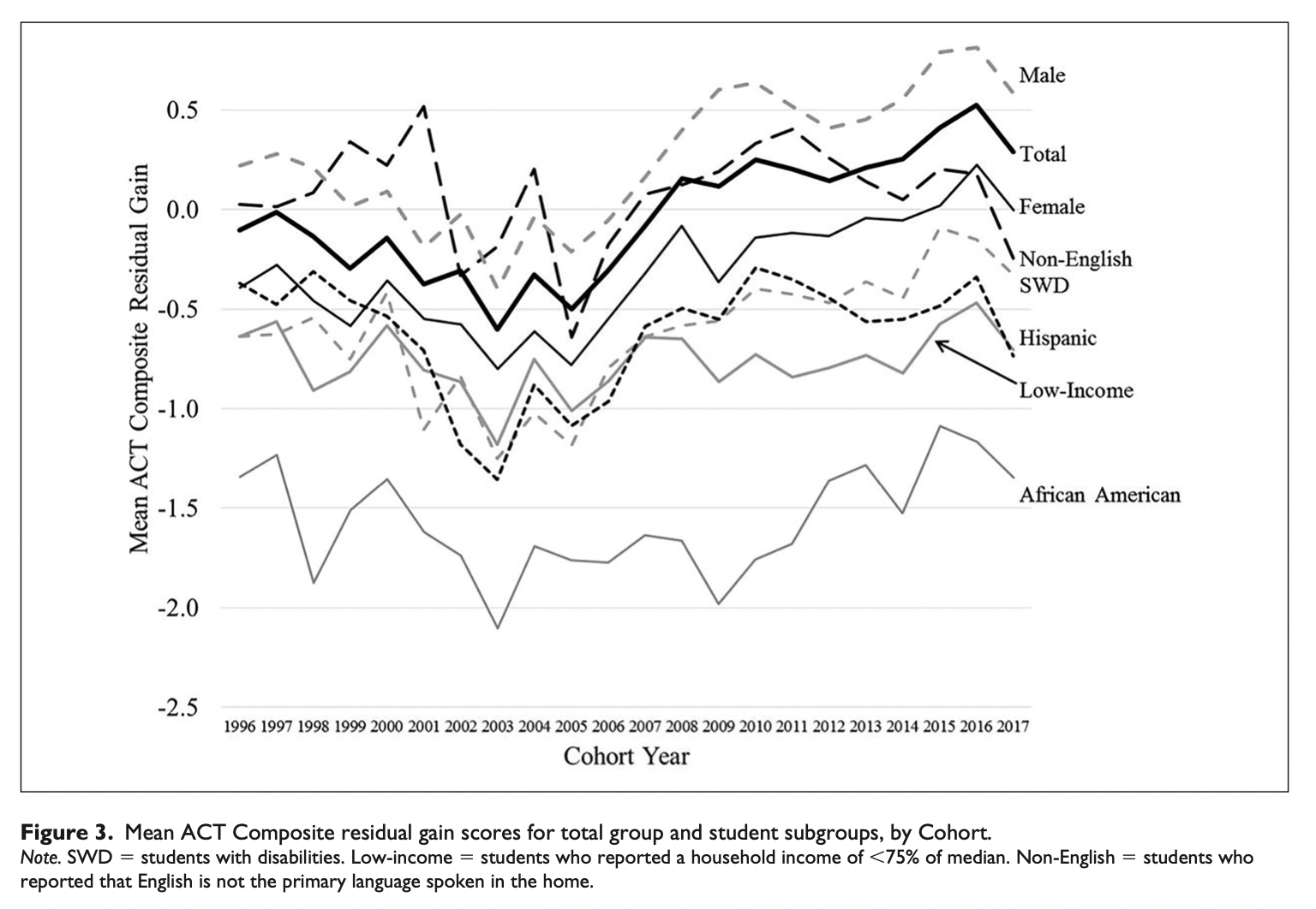
"...To address RQ1, we first plotted the mean growth scores (residual gain ACT Composite scores) by cohort year (Figure 2). By definition, the mean growth score is 0 in the total group. There was a general downward trend in growth from 1996 to 2005, and the mean growth score was at its lowest point (−0.60) for the 2003 cohort. From 2005 to 2017, there was a consistent upward trend in growth, and the mean score was at its highest point (0.53) for the 2016 cohort. Because the trend was different for 1996 to 2004 and 2005 to 2017, we conducted three separate trend tests: 1996 to 2017 (entire study period), 1996 to 2004 (early period of the downward trend), and 2005 to 2017 (later period of the upward trend)...."

What Boots Talent Development? Examining Predictors Of Academic Growth In Secondary School Among Academically Advanced Youth Across 21 Years: Comments Image 3


"... Over the entire study period, mean growth from 7th to 11th/12th grade improved by 0.035 units per year for academically advanced youth (Table 3, p <.001). This improvement can be translated to ACT Composite score points over the entire study period by multiplying the coefficient by the number of years (21), translating to 0.74 (0.035 × 21 years) ACT Composite score points from 1996 to 2017.The improvement can also be translated to an effect size measure, such as Cohen’s d. For example, the standard deviation of ACT Composite scores among all ACT-tested high school graduates is 5.6 (ACT, 2016), so the improvement is comparable to an effect size of about 0.13 (0.74/5.6), which is simi- lar to Cohen’s benchmark for a “small” effect (Cohen, 1988). For the later period (2005-2017), mean growth improved by 0.062 units per year and for the earlier period (1996-2004), mean growth decreased by 0.052 units per year. The results suggest that academic growth from 7th to 11th/12th grade among academically advanced youth has improved over the past two decades, with the improvement occurring over the past 13 years. The average gain (difference score) in ACT Composite score from grade 7 to grade 11/12 was 9 points, which translates to about two points per academic year. This provides a benchmark for comparing the improvement with growth that is typically obtained from one year of instruction: The improvement of 0.74 ACT Composite score points over the 22-year period is comparable to students in 2017 having received an extra 0.37 year of instruction, relative to students in 1996 (calculated as 0.74/2.00)...."

  • Test Scores
  • Workforce
    • Education
      • K-12


Loading More Posts

End of content

No more pages to load

© Copyright 2026 Coherent Research Institute · All Rights Reserved · Privacy · Terms